Conditional formatting

Conditional formatting in a Pivot Table allows you to highlight specific values based on conditions, making it easier to analyze data. Here’s how you can apply conditional formatting in a Pivot Table in Grafieks Cloud.

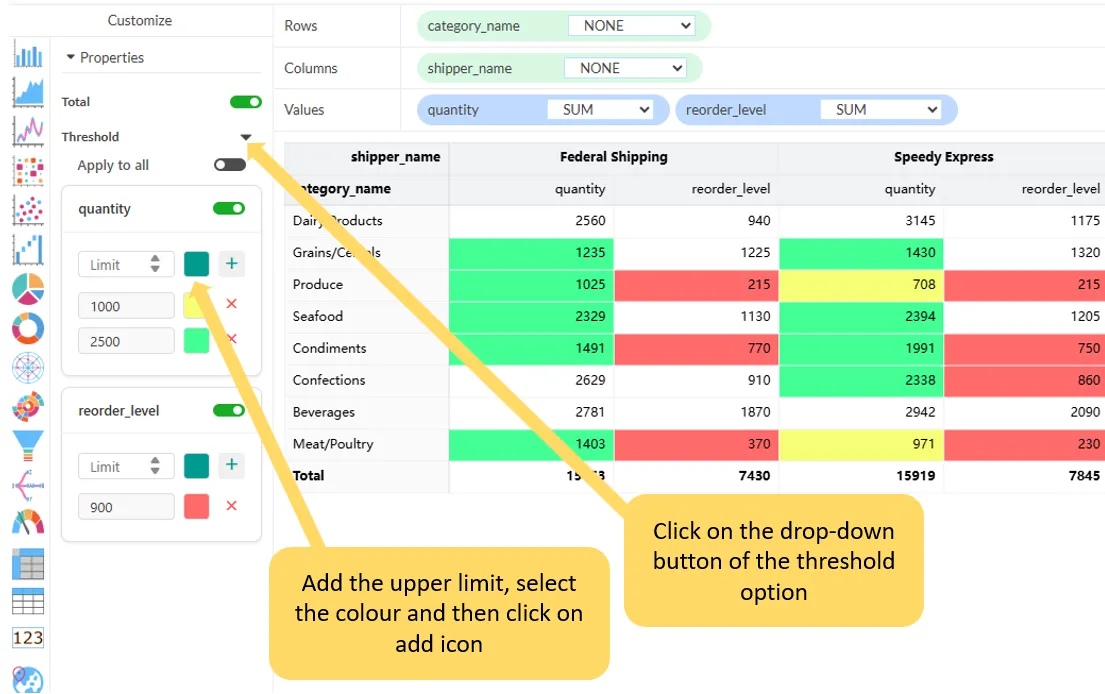
Steps to apply conditional formatting in a pivot table

1. Add required fields to the drop zone
2. Click the dropdown icon in the Threshold menu under the Properties section
3. Enter the upper limit in the input field
4. Choose a color and click the + icon
5. Repeat the steps to add additional limits
6. To apply the same format to other numerical fields, click ‘Apply to all’ or continue with step 7
7. If needed, repeat steps 1–4 for additional numerical fields

Note: The current version supports adding only an upper limit.